Visualizing Celestial Mechanics: N-Body Orbital Resonance in 3D

2026/8/9

The universe is a master of choreography. When multiple celestial bodies interact through gravity, their paths often lock into complex orbital resonances, drawing mathematically perfect mandalas across the cosmos. "Celestial N-Body Orbital Resonance 3D" is a generative physics simulation that attempts to capture this cosmic dance. By placing thousands of digital asteroids in a trinary star system, we can watch as gravity weaves chaotic trajectories into highly structured, glowing celestial mandalas in a dark void.The visual result is an immense, luminous web of orbital paths. Fast-moving particles trace bright cyan arcs, while slower bodies build up dense amber and navy structures. Using Python, the py5 framework, and NumPy's vectorized mathematics, we can compute the gravitational forces for thousands of bodies at 60 frames per second, transforming raw physics into cinematic art.

Visual & Aesthetic Approach

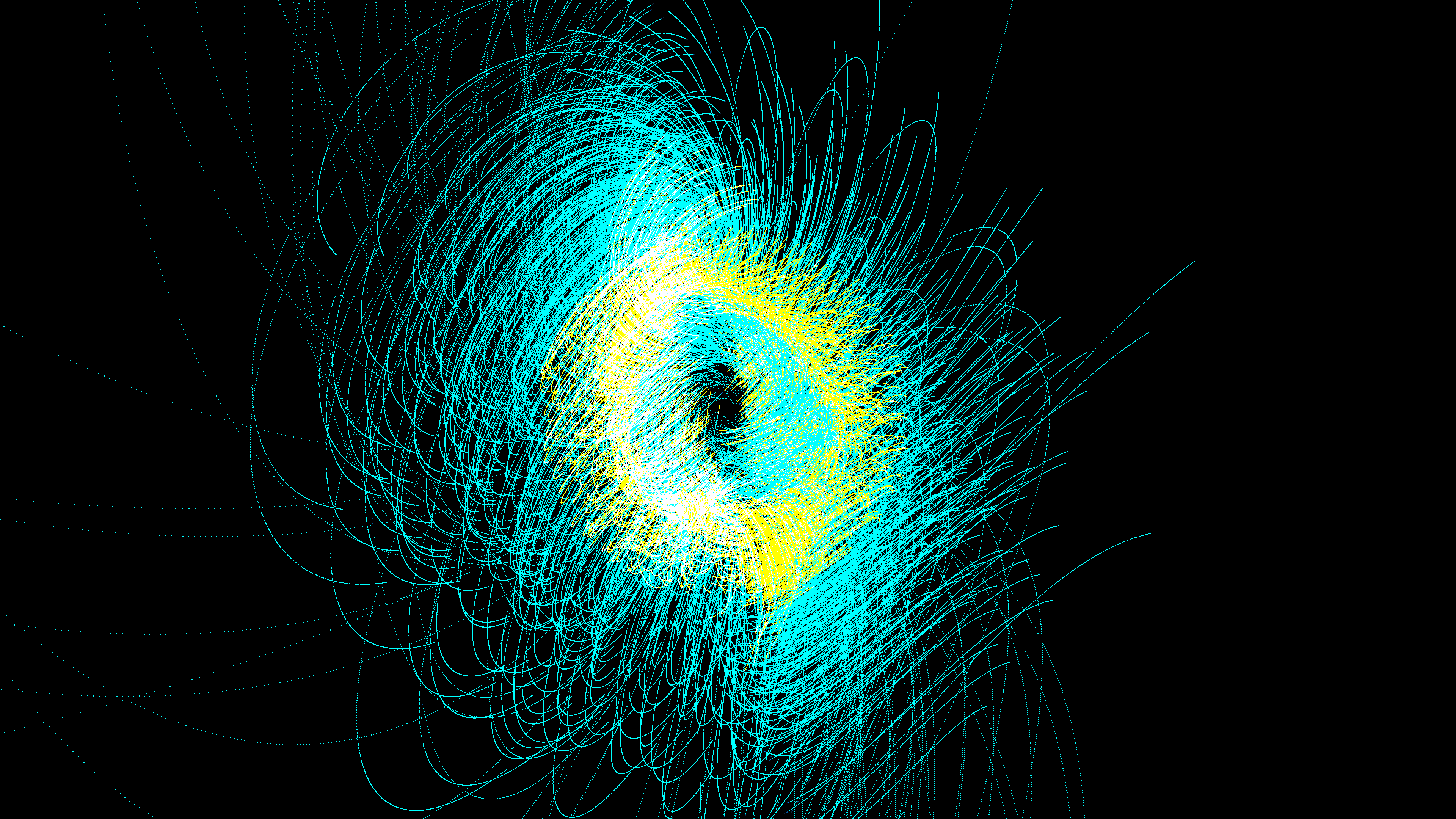
To visualize the concept of "orbital resonance," we need to see the history of a particle's movement, not just its current position. In this simulation, the canvas is cleared to pure black only once at the beginning. Every subsequent frame draws the particles as semi-transparent points using additive blending (py5.blend_mode(py5.ADD)). Over time, these tiny points accumulate to draw thick, glowing trails.

This technique is analogous to long-exposure astrophotography. Because the particles are trapped in the gravitational wells of three massive attractors, their paths naturally fold over themselves. The colors are strictly tied to physics: the speed of the particle dictates its hue. As particles whip around a heavy mass (periapsis), they accelerate and glow a bright, hot cyan. As they drift into the outer void (apoapsis), they slow down, cooling to amber and dark navy. This creates a natural, physically-driven color gradient that highlights the energy states of the system.

Code & Technical Breakdown

At its core, this is a classic N-body simulation, but optimized heavily using NumPy. Instead of looping through particles individually—which would cripple performance in Python—we calculate the gravitational forces across the entire array simultaneously.

Initializing the Trinary System

In the setup() phase, we create 3,000 particles and place them in a slightly flattened 3D disk. We then establish three stationary, massive attractors arranged in an equilateral triangle.

# Initial positions in a flattened disk
positions = np.random.randn(num_particles, 3) * 500
positions[:, 2] *= 0.1 

# Set up 3 heavy central attractors in a triangle to create resonance
R = 400
attractors = np.array([
    [R * np.cos(0), R * np.sin(0), 0],
    [R * np.cos(2*np.pi/3), R * np.sin(2*np.pi/3), 0],
    [R * np.cos(4*np.pi/3), R * np.sin(4*np.pi/3), 0]
])

To ensure the particles orbit rather than simply crashing into the center, we calculate a perpendicular tangent vector for their initial velocities using a cross product, giving the entire system a unified spin.

Vectorized Gravitational Physics

During the draw() loop, we must calculate the pull of every attractor on every particle. We use Newton's law of universal gravitation, but introduce a "softening" parameter to prevent the math from exploding when a particle gets too close to an attractor.

G = 80000.0
dt = 0.05

forces = np.zeros_like(positions)
for attr in attractors:
    # Vectorized distance calculation for all 3000 particles simultaneously
    diff = attr - positions
    
    # 5000.0 is the softening parameter to prevent infinite forces
    dist_sq = np.sum(diff**2, axis=1, keepdims=True) + 5000.0 
    
    # F = G * m1 * m2 / r^2 (mass is 1, so omitted)
    f = G * diff / (dist_sq * np.sqrt(dist_sq))
    forces += f
    
# Euler integration step
velocities += forces * dt
positions += velocities * dt

Because NumPy handles the array operations in highly optimized C code under the hood, this entire physics step evaluates in milliseconds.

Speed-Based Coloring

Finally, we map the magnitude of the velocity vectors to our color palette.

speeds = np.linalg.norm(velocities, axis=1)

py5.begin_shape(py5.POINTS)
for i in range(num_particles):
    s = speeds[i]
    if s > 40:
        py5.stroke(0, 255, 255, 30) # Cyan for high velocity
    elif s > 20:
        py5.stroke(255, 150, 0, 20) # Amber for medium velocity
    else:
        py5.stroke(0, 50, 150, 10)  # Navy for slow velocity
        
    py5.vertex(positions[i, 0], positions[i, 1], positions[i, 2])
py5.end_shape()

celestial n body orbital resonance 3d p1

Conclusion

"Celestial N-Body Orbital Resonance 3D" showcases how strict physical laws can generate profound organic beauty. By relinquishing control to gravity and time, we act as observers to a simulated universe. The overlapping, chaotic paths inevitably find structure, proving that even in a digital void, physics is the ultimate artist.

GitHub: https://github.com/asamiile/py5-media-art/tree/main/sketch/celestial_n_body_orbital_resonance_3d

Purchase assets: Adobe Stock

AI Agent Claude Code Generative Art MCP Server Python