Simulating 3D Solar Flares and Plasma Arcs with py5
2026/8/19
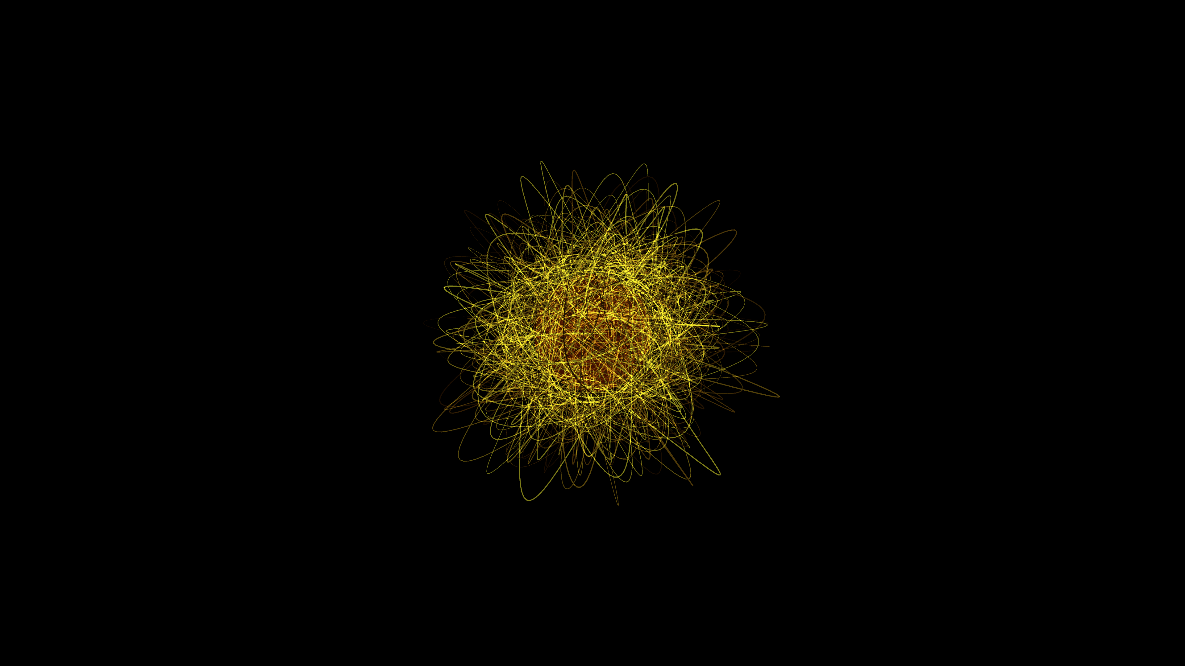
Creating a macro view of a star's surface requires capturing both the immense scale and chaotic energy of solar phenomena. "Kinetic Solar Flare Plasma Arcs 3D" is a generative animation that visualizes massive glowing arcs of plasma erupting violently along invisible magnetic field lines.The visual result is a terrifying and beautiful continuous loop. Deep oranges, intense yellows, and pure white hot spots form a turbulent stellar surface, where thousands of individual strands of plasma twist and pulse outward from a central core. By using py5, a Python-based creative coding framework, we can seamlessly blend complex 3D math and noise functions with efficient rendering to bring this stellar physics simulation to life.
Visual & Aesthetic Approach
The aesthetic goal of this piece is a cinematic, realistic representation of solar turbulence. Rather than relying on standard particle emitters, the plasma arcs are constructed as dense clusters of 3D Bezier curves. These curves provide a smooth, continuous path that mimics the behavior of plasma trapped in magnetic loops.To achieve the glowing, high-energy look of a star, the rendering utilizes additive blending (py5.blend_mode(py5.ADD)). By drawing multiple semi-transparent curves over each other on a pure black background, the intersecting points accumulate brightness naturally, creating intense white-hot cores surrounded by softer orange and red halos. The geometry is driven by high-frequency 3D OpenSimplex noise, which perturb the control points of the curves, ensuring that the plasma never moves uniformly but instead writhes with chaotic turbulence.Code & Technical Breakdown
The core of the simulation relies on precomputing the start and end points of the plasma arcs on the surface of a central sphere, and then dynamically perturbing their control points during the draw loop.Generating the Arc Geometry
Instead of calculating new paths entirely from scratch every frame, we define the base geometry for 1,500 arcs in the setup phase. The endpoints are pushed to the surface of a virtual sphere, while the Bezier control points are extended outward.# Precompute endpoints on a sphere's surface
num_arcs = 1500
arc_starts = np.random.uniform(-400, 400, (num_arcs, 3))
arc_ends = np.random.uniform(-400, 400, (num_arcs, 3))
for arr in (arc_starts, arc_ends):
norms = np.linalg.norm(arr, axis=1, keepdims=True)
# Push points to a radius between 200 and 300
arr[:] = (arr / norms) * np.random.uniform(200, 300, (num_arcs, 1))
# Extend control points outward to create the loop shape
mid_points = (arc_starts + arc_ends) / 2
mid_norms = np.linalg.norm(mid_points, axis=1, keepdims=True)
mid_norms[mid_norms == 0] = 1
arc_cp1 = mid_points + (mid_points / mid_norms) * np.random.uniform(100, 500, (num_arcs, 1))
arc_cp2 = mid_points + (mid_points / mid_norms) * np.random.uniform(100, 500, (num_arcs, 1))This ensures the arcs form natural loops extending away from the core, mimicking magnetic field lines that break the star's surface.
Animating with Noise and Sine Waves
During the draw loop, we apply both an absolute sine wave pulse to control visibility and intensity, and OpenSimplex noise to introduce spatial turbulence.phase = arc_phases[i] + t * py5.TWO_PI * 2.0
# Pulse intensity based on a sine wave
intensity = py5.sin(phase)
if intensity > 0:
# Map intensity to HSB colors (Deep Red to Hot Yellow)
hue = 20 + intensity * 40
sat = 100 - intensity * 20
brightness = 60 + intensity * 40
alpha = 10 + intensity * 40
py5.stroke(hue, sat, brightness, alpha)
# Apply noise to control points for turbulence
noise_val1 = py5.os_noise(arc_cp1[i,0]*0.01, arc_cp1[i,1]*0.01, arc_cp1[i,2]*0.01 + t*5) * 100
noise_val2 = py5.os_noise(arc_cp2[i,0]*0.01, arc_cp2[i,1]*0.01, arc_cp2[i,2]*0.01 + t*5) * 100
c1x, c1y, c1z = arc_cp1[i] + noise_val1
c2x, c2y, c2z = arc_cp2[i] + noise_val2
p1x, p1y, p1z = arc_starts[i]
p2x, p2y, p2z = arc_ends[i]
# Draw the dynamic plasma arc
py5.begin_shape()
py5.vertex(p1x, p1y, p1z)
py5.bezier_vertex(c1x, c1y, c1z, c2x, c2y, c2z, p2x, p2y, p2z)
py5.end_shape()By adding the time variable t into the Z-axis of the noise function (t*5), we drag the 3D noise field through the control points over time. This causes the arcs to writhe organically without losing their fundamental shape. The dynamic HSB color mapping ensures that as an arc pulses closer to its peak intensity, it naturally heats up from a dim red to a blinding yellow-white.