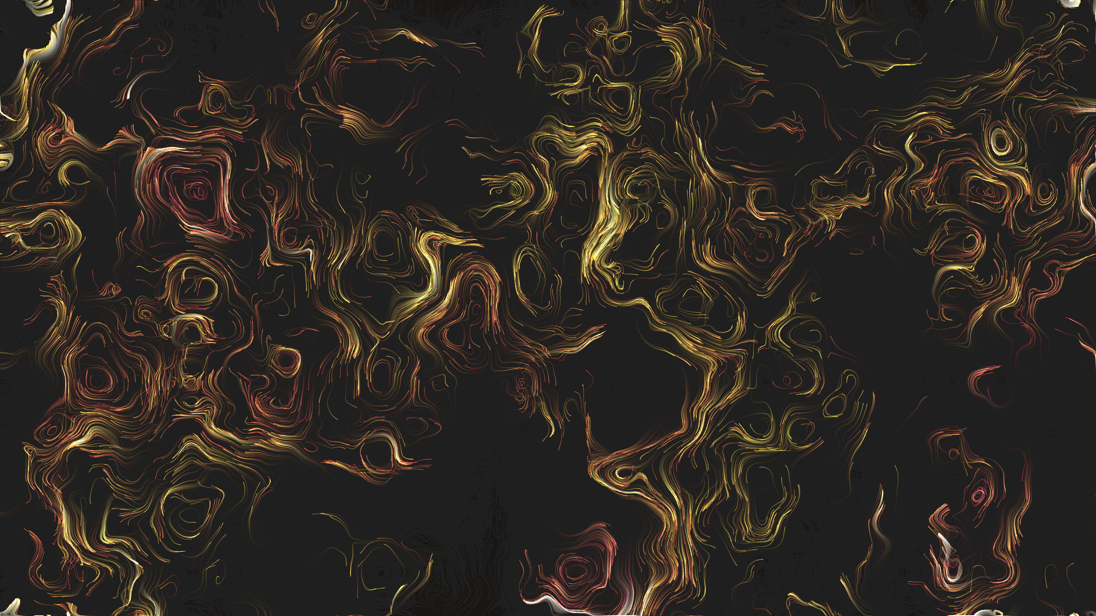
Neon Topography: Tracing Contour Flows with Py5 and Noise Gradients
2026/8/31
Generative art often finds its most compelling aesthetics when modeling mathematical structures hidden in nature. My latest piece, a generative topographic map, visualizes an unseen terrain where 15,000 glowing particles continuously trace the contour lines of a slowly shifting 3D Perlin noise landscape.Imagine looking down at a dark void where electric purple and bright pink streams of light flow seamlessly, mapping out invisible mountains and valleys. The streams weave intricately alongside one another without intersecting, leaving glowing trails that gradually build up into complex, shifting topographical rings and fluid structures. It’s an exercise in visualizing vector fields with high density.Python and the py5 library proved to be the ideal tooling for this particular concept. Calculating vector gradients and updating physics for thousands of particles on a frame-by-frame basis requires robust math operations, which Python's NumPy handles gracefully. Py5 then provides the pristine canvas and additive blending operations needed to transform these raw coordinates into cinematic, glowing streaks of light.
Visual & Aesthetic Approach
The core technique behind this animation is the computation of a 2D gradient from a continuously evolving Perlin noise field. By finding the direction of the steepest ascent (the gradient) and rotating those vectors by 90 degrees, the particles flow perfectly perpendicular to the slope. This means they perpetually trace the contour lines of the noise terrain.To achieve the "Neon Topography" look, I employed py5's ADD blend mode alongside a semi-transparent black fade drawn over the canvas each frame. As particles move, their glowing trails overlap and accumulate brightness, simulating long-exposure photography. The palette revolves around electric purples and bright pinks, which dynamically shift depending on the underlying noise elevation, bringing a deep-sea luminescence and high-tech cinematic tone to the piece.Code & Technical Breakdown
The heavy lifting happens within the draw loop, where we calculate the noise field, derive its gradients, and update our 15,000 particles. To keep performance manageable, a lower-resolution noise grid is precomputed and its gradients are extracted using NumPy.# Precompute noise grid for fast gradient lookup
grid_res = 10
cols = py5.width // grid_res + 2
rows = py5.height // grid_res + 2
noise_grid = np.zeros((rows, cols), dtype=np.float32)
for r in range(rows):
for c in range(cols):
noise_grid[r, c] = py5.noise(c * grid_res * noise_scale, r * grid_res * noise_scale, time_val)
# Compute gradients of the grid
dy, dx = np.gradient(noise_grid)By computing np.gradient, we immediately get the dx and dy matrices representing the slope across the entire canvas. Next, we map our particle coordinates to this grid and calculate their velocities:
# Map particle positions to grid indices
c_idx = (pos[:, 0] / grid_res).astype(np.int32)
r_idx = (pos[:, 1] / grid_res).astype(np.int32)

# Get gradient
grad_x = dx[r_idx, c_idx]
grad_y = dy[r_idx, c_idx]

# Vector perpendicular to gradient traces the contour line: (-grad_y, grad_x)
vx = -grad_y
vy = grad_x

# Normalize velocity
v_mag = np.sqrt(vx**2 + vy**2) + 0.0001
vx = (vx / v_mag) * dt
vy = (vy / v_mag) * dt
This simple 90-degree rotation (-grad_y, grad_x) is the mathematical heart of the sketch. It takes vectors pointing straight uphill and turns them sideways. The particles are thus locked into traversing the ridges and valleys of the noise space.Finally, we translate the abstract math into the neon aesthetic by tying particle color directly to the underlying noise field:
# Color shifts based on local noise value to highlight contours
local_noise = noise_grid[r_idx[i], c_idx[i]]
# 280 (purple) to 340 (pink) + noise mapping
hue = (hues[i] + local_noise * 100 + time_val * 20) % 360

# Additive drawing with low opacity
py5.stroke(hue, 80, 90, 40)
py5.line(pos[i, 0], pos[i, 1], new_x[i], new_y[i])
Py5’s HSB color mode allows us to smoothly shift hues. By adding the local_noise and an advancing time_val to the base hue, the topographical map gains an extra dimension of visual depth, smoothly rippling through the purple and pink spectrum as the landscape evolves.