Orbiting the Abyss: Simulating a Binary Black Hole Accretion Disk in Python
2026/9/2
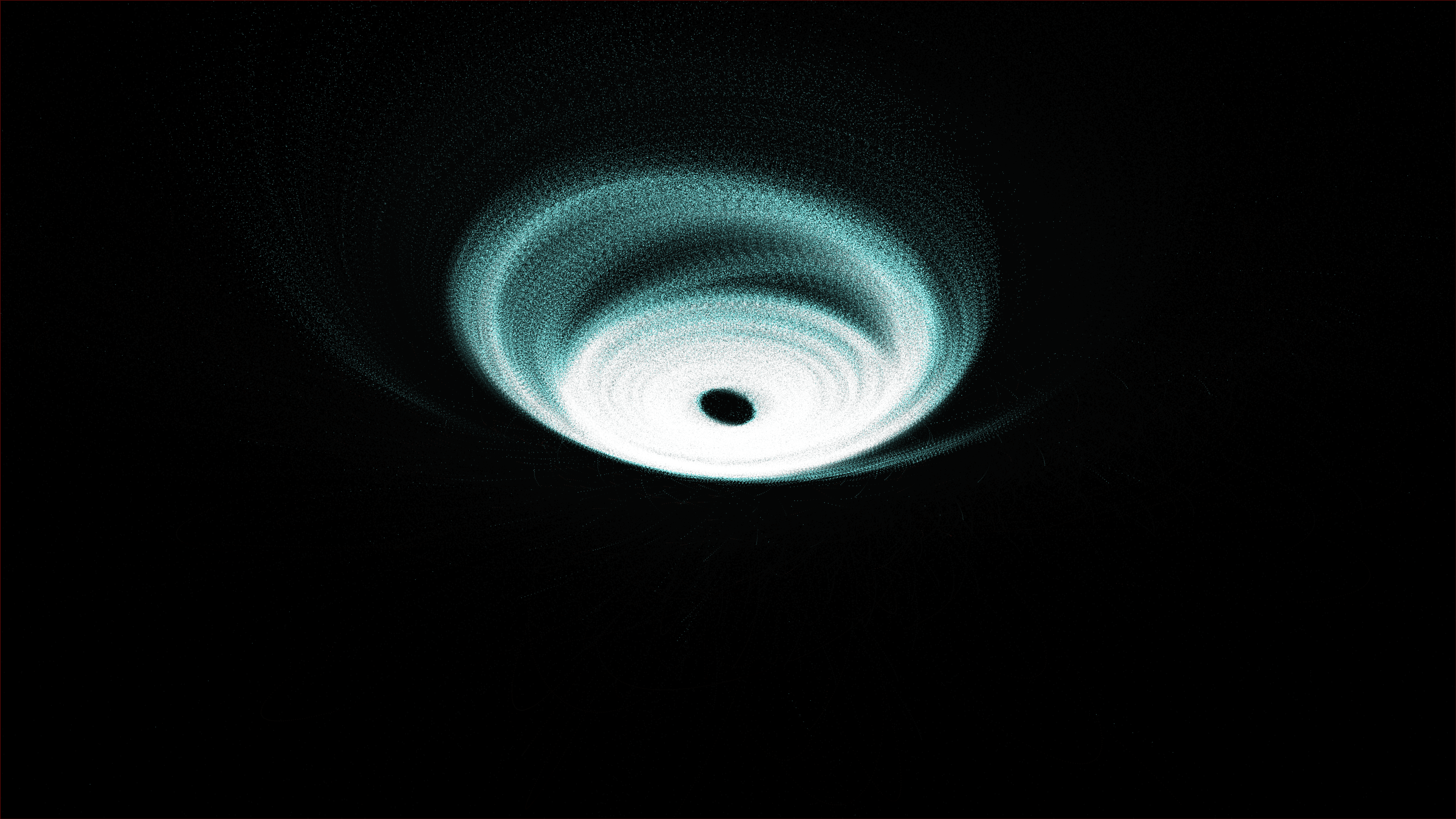
Generative art thrives at the intersection of complex mathematics and visual beauty. My recent work, an interactive physics simulation, visualizes a massive accretion disk swirling around a binary black hole system. By tracking the orbital mechanics of 150,000 glowing particles, the sketch captures the chaotic, high-energy environment of cosmic singularities.Imagine gazing down at an isometric cross-section of deep space. Two immense, invisible gravitational bodies perform a slow orbital dance, tearing through a vast disk of cosmic dust. The particles streak across the screen in sweeping arcs, glowing in blistering whites, yellows, and oranges near the event horizons, while cooler, slower matter drifts away in deep reds and cyans.Python and the py5 library provide the perfect environment for this kind of simulation. Running gravity calculations for 150,000 independent bodies would cripple a standard for loop, but Python’s NumPy library allows us to vectorize the physics engine, calculating the forces in a fraction of a second. Py5 then handles the massive point-cloud rendering, utilizing additive blending to create the volumetric, glowing density of a true accretion disk.
Visual & Aesthetic Approach
The animation relies on an O(N) gravity calculation where every particle is pulled by two central, moving point masses. Instead of calculating the gravitational pull between every single particle (which would be an $O(N^2)$ operation and far too slow), the simulation treats the black holes as the only significant sources of gravity.The palette of the piece is deeply tied to the physics. To simulate the extreme thermal energy and relativistic Doppler beaming (blueshifting/redshifting) seen in real accretion disks, the color of each particle is mapped directly to its scalar speed. Particles whipping around the event horizon glow with intense white and cyan energy, while those on the outer edges or being ejected burn in cooler oranges and deep, fading reds.The tone is explicitly cinematic and realistic, stripping away stylized elements to focus purely on the raw, mathematical beauty of orbital mechanics.Code & Technical Breakdown
The core of the simulation lies in how we calculate the gravitational pull from the two moving singularities. We define their positions dynamically using trigonometric functions to simulate an orbit, then calculate the force vectors for all 150,000 particles at once.# Binary black hole positions
orbit_r = 50.0
bh1 = np.array([np.cos(time_val)*orbit_r, 0, np.sin(time_val)*orbit_r])
bh2 = np.array([-np.cos(time_val)*orbit_r, 0, -np.sin(time_val)*orbit_r])
M1, M2 = 1000.0, 1000.0
# Calculate gravity force from BH1 (Vectorized)
d1 = bh1 - positions
dist1_sq = np.sum(d1**2, axis=1) + 100.0 # Softening parameter to prevent infinity
dist1 = np.sqrt(dist1_sq)
f1_mag = (G * M1) / dist1_sq
f1 = (d1 / dist1[:, np.newaxis]) * f1_mag[:, np.newaxis]A crucial detail here is the + 100.0 softening parameter added to dist1_sq. In orbital simulations, if a particle passes exactly through the center of a mass, the distance becomes zero, causing the gravitational force to shoot to infinity and breaking the simulation. Softening prevents these singularities from causing numerical explosions.Once we update the velocities and positions based on these forces, we need to handle particles that inevitably fall into the black holes or get flung too far away:
# Event horizon (destroy and respawn particles that get too close or too far)
too_close = (dist1 < 10) | (dist2 < 10) | (np.sum(positions**2, axis=1) > 1000000)
if np.any(too_close):
    num_respawn = np.sum(too_close)
    new_radii = np.random.uniform(350, 400, num_respawn)
    new_angles = np.random.uniform(0, 2 * np.pi, num_respawn)

    # Respawn at the outer edge of the disk
    positions[too_close, 0] = np.cos(new_angles) * new_radii
    positions[too_close, 2] = np.sin(new_angles) * new_radii
    positions[too_close, 1] = np.random.normal(0, 5, num_respawn)
By constantly recycling the "dead" particles back into the outer edges of the accretion disk, we ensure the simulation can run indefinitely without the disk eventually draining into the void.Finally, to render the particles, we use a custom 3D rotation matrix and perspective projection to convert the 3D space into py5's 2D canvas. We then group the particles by their calculated speed to apply different strokes in batches, which is vastly more efficient than changing the stroke color per-particle.
# Color by speed (blueshift / redshift proxy)
speed = np.sqrt(np.sum(velocities**2, axis=1))[valid_z]

# Fast particles (White / Cyan)
fast_mask = speed > 15.0
if np.any(fast_mask):
    py5.stroke(180, 50, 100, 40)
    py5.points(np.column_stack((proj_x[fast_mask], proj_y[fast_mask])))