Visualizing Sound: Procedural Chladni Resonance Patterns with Python
2026/9/8
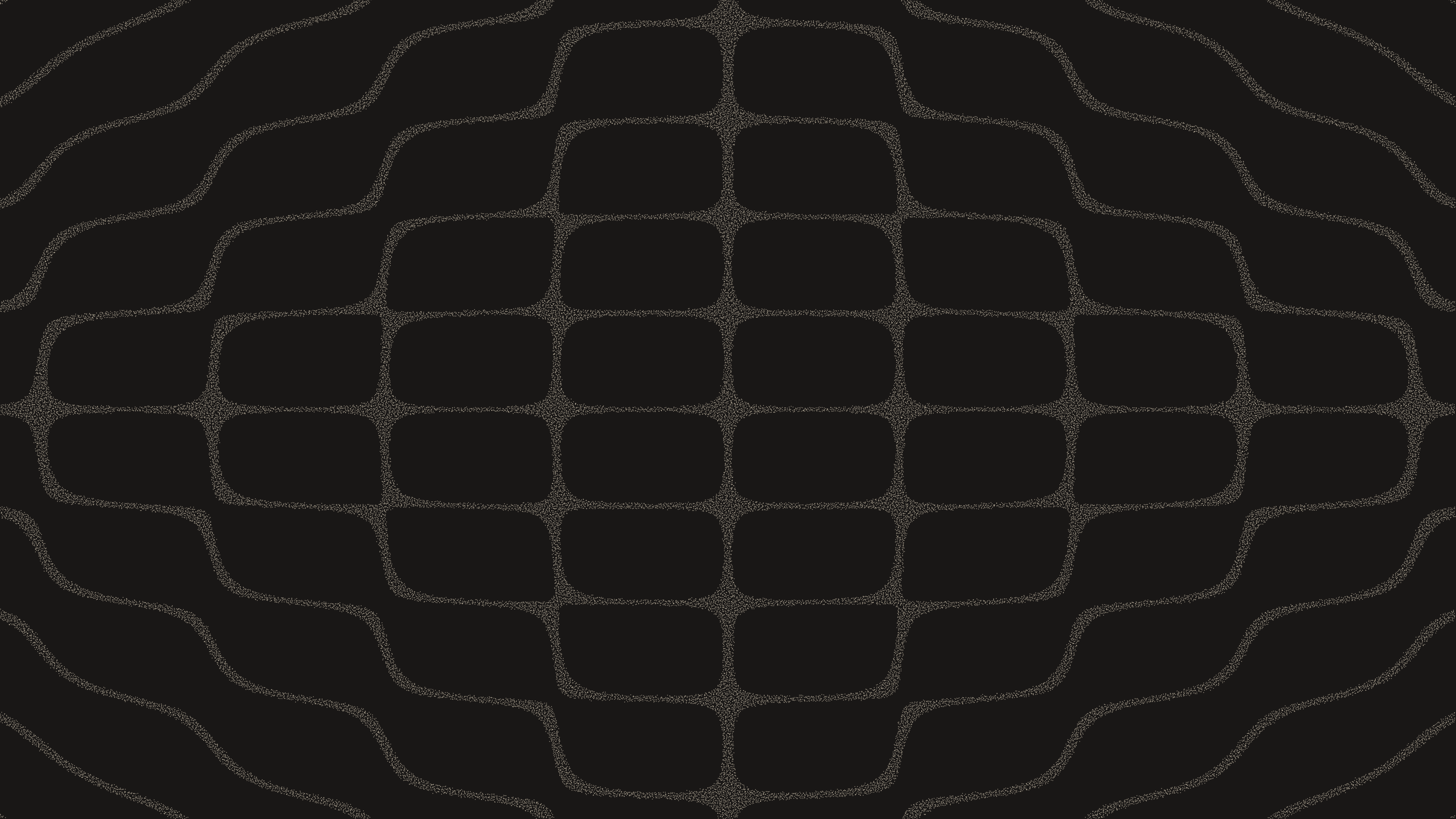
Creative coding allows us to simulate the invisible forces of nature. In this sketch, Kinetic Chladni Resonance Patterns, I aimed to recreate the mesmerizing phenomenon of Chladni figures—patterns formed when a physical plate is vibrated at resonant frequencies, causing scattered sand to collect at the stationary nodes of the resulting standing waves.Visually, the result is both organic and highly mathematical. Monochromatic, off-white "sand grains" continuously vibrate and shift across a dark, warm-brown surface, spontaneously organizing themselves into intricate, symmetrical mandalas before breaking apart and forming new structures. To achieve this, I used py5 for rendering and relied heavily on NumPy for evaluating complex trigonometric functions across a dense 2D grid. The performance requirements of doing this per-frame are immense, making NumPy's vectorized operations absolutely essential for the simulation.
Visual & Aesthetic Approach
The aesthetic goal was to maintain physical realism without sacrificing geometric purity. Real sand on a vibrating plate doesn't form perfect, razor-sharp lines; it gathers in slightly scattered, organic ridges. To emulate this, the palette is intentionally restrained—a dark, muted brown background acting as the acoustic plate, contrasted by high-opacity, off-white points representing the sand. By extracting the mathematical nodes of the standing wave equation and applying a tiny amount of Gaussian jitter to each point, the resulting lines appear sharp from a distance but granular and natural up close.Code & Technical Breakdown
Simulating this effect requires two primary steps: generating a dense mesh of coordinates to evaluate the standing wave, and applying the mathematical equation to find the resting nodes.1. Vectorized Grid Generation and the Chladni Equation
Iterating through every pixel on a 4K canvas using standard Python loops would reduce the frame rate to a crawl. Instead, we generate a normalized coordinate grid upfront using NumPy, allowing us to evaluate the equation across the entire canvas simultaneously.The heart of the simulation is the 2D standing wave equation:# Ensure time drives smooth transitions between resonant modes
t = py5.frame_count / TOTAL_FRAMES
# Smoothly interpolate the m and n resonance parameters
m = py5.remap(math.sin(t * py5.TWO_PI), -1, 1, 2.0, 7.0)
n = py5.remap(math.cos(t * py5.TWO_PI), -1, 1, 4.0, 9.0)
# Evaluate the Chladni standing wave equation over the normalized grid (X, Y)
# v = a * sin(n * pi * x) * sin(m * pi * y) + b * sin(m * pi * x) * sin(n * pi * y)
term1 = np.sin(n * np.pi * X) * np.sin(m * np.pi * Y)
term2 = np.sin(m * np.pi * X) * np.sin(n * np.pi * Y)
# Modulate a and b to break perfect symmetry slightly over time
a = 1.0
b = 1.0 + math.sin(t * py5.TWO_PI * 2.0) * 0.2
V = a * term1 + b * term2In this block, V represents the vibrational amplitude of the plate at every point (X, Y). By continuously animating the m and n variables, we simulate the effect of sweeping a frequency generator, causing the simulated plate to transition smoothly between different resonant modes.
2. Thresholding and Organic Jitter
Sand naturally bounces off the parts of the plate that are vibrating heavily (antinodes) and settles where the plate is stationary (nodes). Mathematically, this means the sand gathers where V is close to zero.# The sand gathers where V is close to 0 (the nodes)
threshold = 0.15 # Determines the width of the sand lines
mask = np.abs(V) < threshold
# Get the coordinates where the mask is true (the nodes)
sand_x = X_coords[mask]
sand_y = Y_coords[mask]
# Add a tiny bit of random jitter to the sand to make it look organic
jitter_x = np.random.normal(0, 1.5, size=sand_x.shape)
jitter_y = np.random.normal(0, 1.5, size=sand_y.shape)
# Stack the arrays for bulk drawing
points_to_draw = np.column_stack((sand_x + jitter_x, sand_y + jitter_y))
py5.stroke(40, 15, 90, 200) # Off-white sand color
py5.stroke_weight(2)
# Draw all sand grains in one highly efficient call
if len(points_to_draw) > 0:
py5.points(points_to_draw)
Instead of looping through the boolean mask, NumPy's advanced indexing (X_coords[mask]) instantly extracts only the points resting on the nodal lines. We then apply np.random.normal to inject a slight Gaussian displacement. Finally, py5.points() draws the entire array of thousands of particles in a single optimized pass.