Simulating High-Velocity Plasma Streams with Curl Noise in Python
2026/9/14
Creative coding is at its best when it merges complex mathematical concepts with striking visual aesthetics. In my recent sketch, Kinetic Fluid Turbulence Ribbons, I set out to simulate the violent, chaotic energy of high-velocity plasma streams colliding in a magnetic chamber.
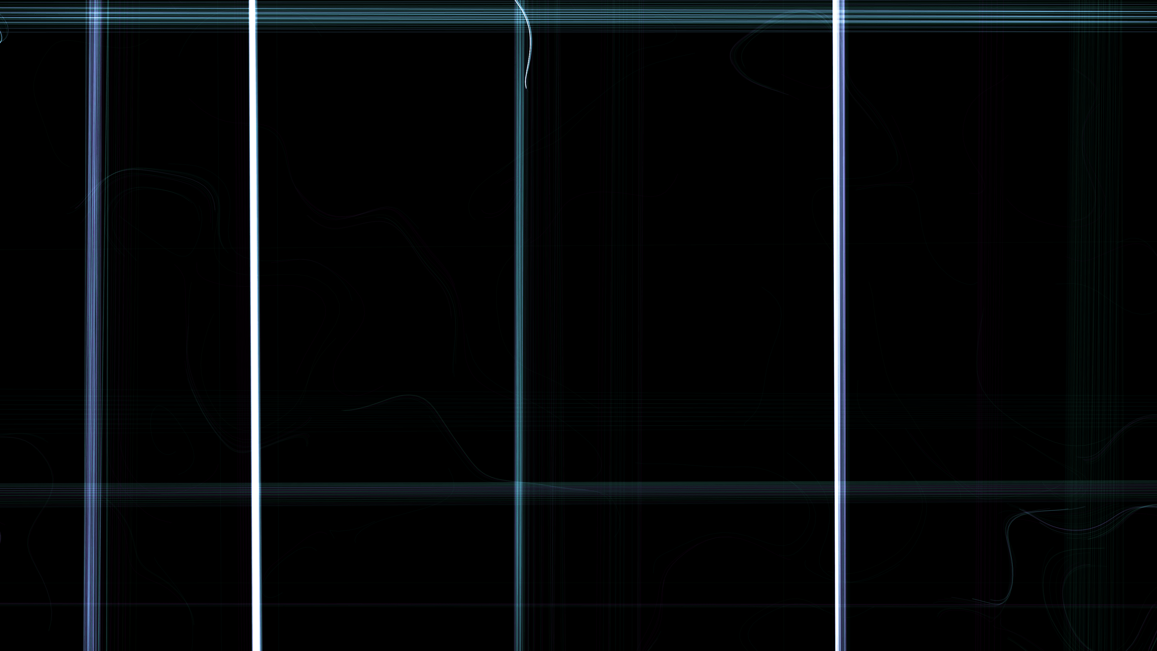
Visually, the piece is intense: glowing neon ribbons of cyan, electric magenta, and bright lime green violently stretch, twist, and tear across a pitch-black void. To achieve this fluid-like, incompressible motion without the heavy computational overhead of a true Navier-Stokes fluid simulation, I turned to curl noise. Paired with Python's NumPy for rapid matrix operations and py5 for high-performance rendering and additive blending, we can create incredibly dense, cinematic particle systems running smoothly in real-time.
Visual & Aesthetic Approach
The aesthetic goal was to capture the sheer power and velocity of plasma. To do this, I needed the particles to leave persistent, glowing trails rather than just appearing as standalone points. By maintaining a history buffer for every particle, we can draw them as continuous, flowing ribbons that fade smoothly into the darkness. Additive blending (py5.blend_mode(py5.ADD)) is critical here. When multiple translucent ribbons overlap in dense, chaotic eddies, their color values accumulate, creating brilliant, blown-out hotspots that perfectly mimic the blinding light of superheated plasma.Code & Technical Breakdown
The core of this simulation hinges on two techniques: calculating divergence-free curl noise, and efficiently managing the particle history buffers for drawing the ribbons.1. Generating Incompressible Flow with Curl Noise
Standard Perlin or OpenSimplex noise can look organic, but it lacks the physical characteristics of a fluid. Particles driven directly by noise tend to converge into "sinks" or get stuck. Fluids, however, are largely incompressible—they flow *around* each other in continuous loops and eddies. To achieve this, we can calculate the curl of the noise field using finite differences:def get_curl(x, y, t):
eps = 0.1
# Sample the noise field around the target point
n1 = py5.os_noise(x, y + eps, t)
n2 = py5.os_noise(x, y - eps, t)
n3 = py5.os_noise(x + eps, y, t)
n4 = py5.os_noise(x - eps, y, t)
# Calculate partial derivatives
a = (n1 - n2) / (2 * eps)
b = (n3 - n4) / (2 * eps)
# The curl is the cross derivative
return np.array([a, -b])By taking the partial derivatives of the noise field in the X and Y directions, and then swapping and negating them, we generate a vector field that has zero divergence. When particles are pushed by this vector field, they naturally form the swirling, eddying structures characteristic of turbulent fluids.
2. High-Performance Ribbon Buffers with NumPy
To draw continuous ribbons, each of the 800 particles must remember its last 30 positions. Doing this with standard Python lists in a for loop would cripple the frame rate. Instead, NumPy allows us to shift the entire history buffer in a single, lightning-fast operation.# Shift the entire history buffer back by one frame for all ribbons simultaneously
for i in range(n_ribbons):
ribbons_x[i, 1:] = ribbons_x[i, :-1]
ribbons_y[i, 1:] = ribbons_y[i, :-1]
hx, hy = ribbons_x[i, 0], ribbons_y[i, 0]
# Calculate the new head position using the curl noise field
curl = get_curl(hx * 0.002, hy * 0.002, t)
hx += curl[0] * 12
hy += curl[1] * 12
# Update the head of the ribbon
ribbons_x[i, 0] = hx
ribbons_y[i, 0] = hyWith the geometry calculated, drawing the ribbons becomes a matter of iterating through the buffer and applying a fading alpha gradient.
py5.begin_shape()
for j in range(tail_length):
    # Fade the tail out smoothly
    alpha = int(py5.remap(j, 0, tail_length, 255, 0))
    py5.stroke(c[0], c[1], c[2], alpha)
    py5.vertex(ribbons_x[i, j], ribbons_y[i, j])
py5.end_shape()
This combination of py5.begin_shape() and mapped alpha values yields the smooth, neon-tube aesthetic that defines the piece.