Simulating Swirling Fluid Dynamics with Perlin Noise in Python
2026/9/16
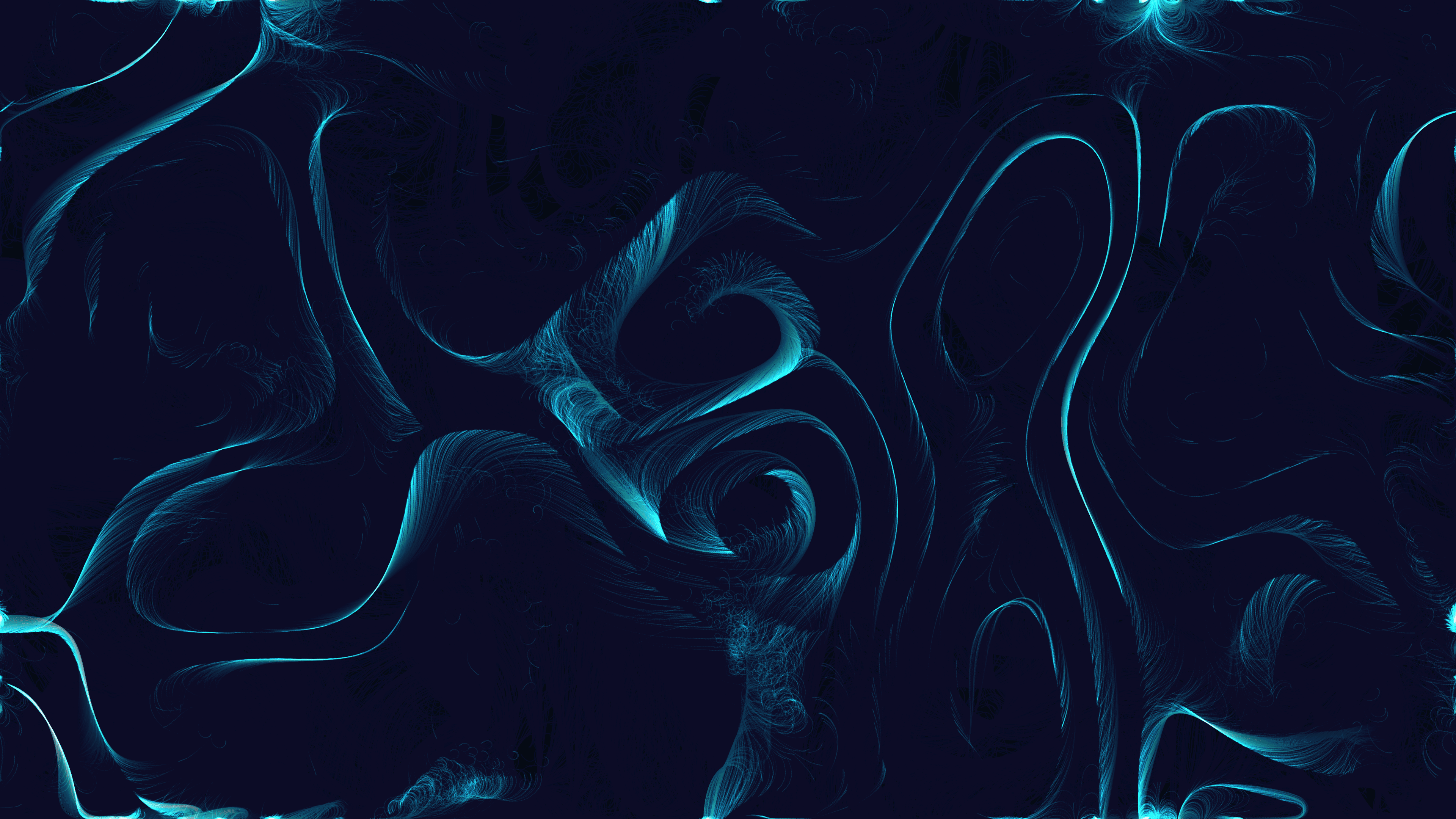
In creative coding, some of the most compelling visuals emerge from simulating the chaotic, yet structured, flow of nature. In this sketch, Kinetic Fluid Dynamics Particles, I set out to simulate the mesmerizing movement of fluid dynamics. By deploying 15,000 individual particles into a procedurally generated vector field, the script captures the essence of swirling, turbulent water.Visually, the result is dense and cinematic. Thousands of glowing, oceanic-hued particles—ranging from bright aqua to deep teal—flow across a dark indigo canvas, leaving fading trails of light in their wake. Python, powered by the high-performance numerical operations of NumPy and the creative coding framework py5, is the perfect environment for this. It allows us to efficiently manage the kinematics of tens of thousands of particles in real-time, resulting in a buttery-smooth, high-resolution simulation.
Visual & Aesthetic Approach
The aesthetic goal was to evoke the feeling of looking into a deep, bioluminescent ocean current. Rather than rendering rigid shapes, the focus is entirely on the motion and history of the particles. To achieve this, the simulation relies on persistent, fading trails rather than clearing the screen completely each frame. By combining this technique with additive blending (py5.blend_mode(py5.ADD)), the areas where particles congregate and overlap become brilliantly illuminated, mimicking the density and energy of a high-pressure fluid eddy. The color palette remains strictly within deep oceanic hues, contrasting sharply with the deep indigo void to create a sense of vast depth.Code & Technical Breakdown
Simulating 15,000 particles efficiently requires stepping away from traditional Python for loops where possible and utilizing NumPy for state initialization, combined with a highly optimized draw loop.1. Vector Fields and Particle Kinematics
The fluid motion is driven by a vector field generated using Perlin noise. By sampling a 3D noise space (where the Z-axis is time), we can assign an angle of velocity to every point on the 2D canvas.# Initialize 15,000 particles and their unique speeds
num_particles = 15000
noise_scale = 0.001
noise_z = 0
particles = np.zeros((num_particles, 2))
particles[:, 0] = np.random.uniform(0, py5.width, num_particles)
particles[:, 1] = np.random.uniform(0, py5.height, num_particles)
speeds = np.random.uniform(2, 8, num_particles)In the draw() loop, each particle checks the noise field at its current location to determine which way the "current" is flowing.
# Inside the draw loop for each particle
x = particles[i, 0]
y = particles[i, 1]

# Calculate vector field angle using Perlin noise
angle = py5.os_noise(x * noise_scale, y * noise_scale, noise_z) * py5.TWO_PI * 4

# Move particle based on the angle and its individual speed
nx = x + np.cos(angle) * speeds[i]
ny = y + np.sin(angle) * speeds[i]
By multiplying the noise output by py5.TWO_PI * 4, we allow the angles to wrap multiple times, creating tight, swirling vortices rather than gentle, sweeping curves.
2. Creating Fading Trails with Alpha Blending
To create the signature long, glowing trails without keeping a massive history buffer for every particle, we use a classic generative art trick: drawing a highly transparent rectangle over the entire canvas every frame.def draw():
global noise_z
# Slight fade for trails using a dark rect with very low alpha
py5.blend_mode(py5.BLEND)
py5.fill(5, 10, 20, 10) # Matches the deep indigo background, 10/255 opacity
py5.no_stroke()
py5.rect(0, 0, py5.width, py5.height)
# Switch to additive blending for drawing the luminous particles
py5.blend_mode(py5.ADD)
py5.stroke_weight(2)This effectively "dims" the previous frames slightly, leaving a fading history of where the particles have been. We then draw the current frame's movement as a line segment between the old position and the new position.
    # Draw line segment for trail
    py5.stroke(color_r[i], color_g[i], color_b[i], 30)
    py5.line(x, y, nx, ny)

    # Update state
    particles[i, 0] = nx
    particles[i, 1] = ny

# Animate the noise field slowly in the Z dimension
noise_z += 0.003
By advancing noise_z slightly each frame, the entire vector field shifts and morphs, ensuring that the fluid dynamics never repeat and the particles are constantly driven into new, organic patterns.